

Matrices and graphs
Matrices and graphs
The single most undervalued fact of linear algebra: matrices are graphs, and graphs are matrices

The single most undervalued fact of linear algebra: matrices are graphs, and graphs are matrices.

Encoding matrices as graphs is a cheat code, making complex behavior simple to study.
Let me show you how!
The directed graph of a nonnegative matrix
If you looked at the example above, you probably figured out the rule.
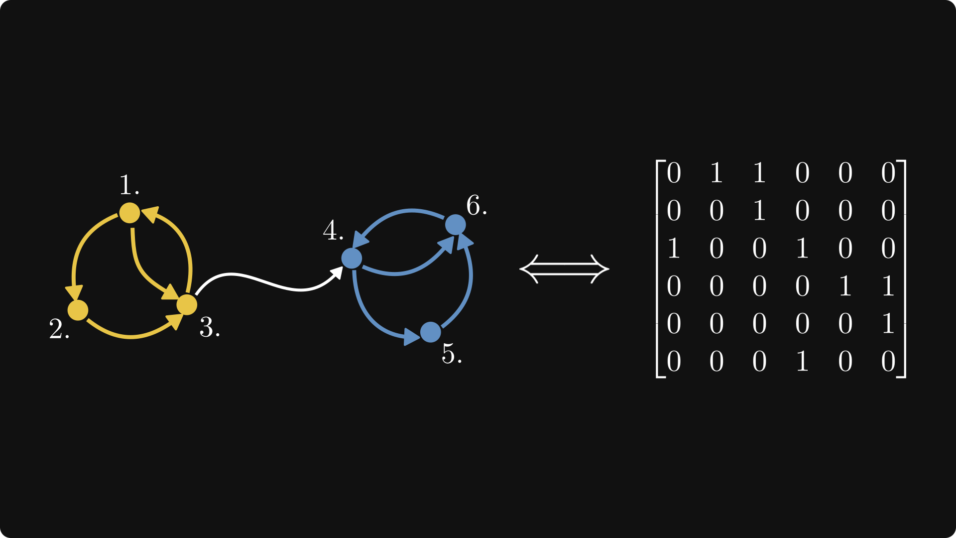
Each row is a node, and each element represents a directed and weighted edge. Edges of zero elements are omitted. The element in the i-th row and j-th column corresponds to an edge going from i to j.
The resulting graph is called the directed graph (or digraph) of the matrix.
To unwrap the definition a bit, let's check the first row, which corresponds to the edges outgoing from the first node.

Similarly, the first column corresponds to the edges incoming to the first node.
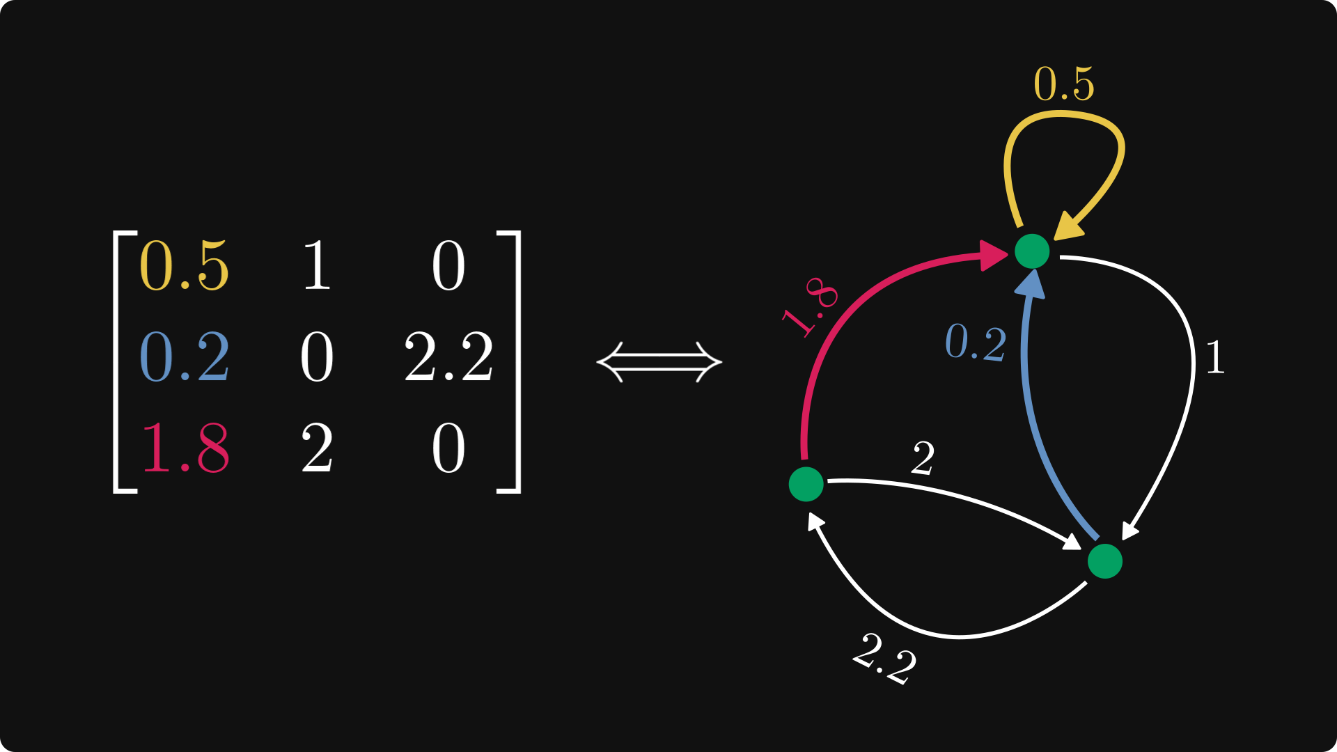
Here is the full picture, with the nodes explicitly labeled.

Benefits of the graph representation
Why is the directed graph representation beneficial for us?
For one, the powers of the matrix correspond to walks in the graph.
Take a look at the elements of the square matrix. All possible 2-step walks are accounted for in the sum defining the elements of A².
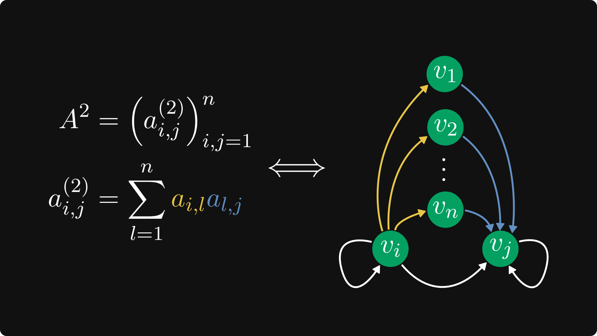
If the directed graph represents the states of a Markov chain, the square of its transition probability matrix essentially shows the probability of the chain having some state after two steps.
There is much more to this connection.
For instance, it gives us a deep insight into the structure of nonnegative matrices.
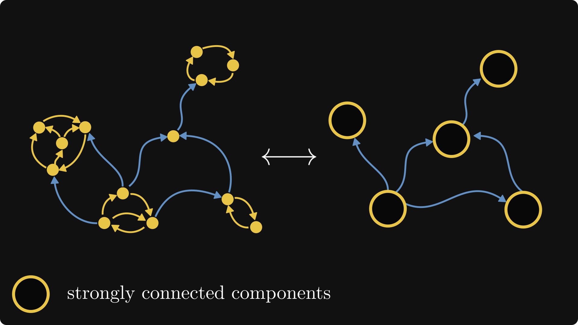
To see what graphs show about matrices, let's talk about the concept of strongly connected components.
The connectivity of graphs
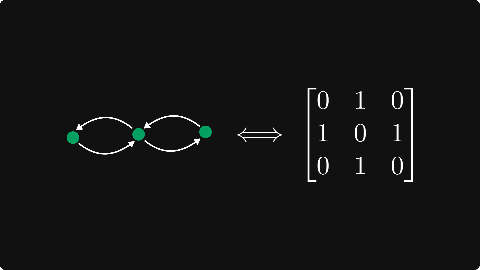
A directed graph is strongly connected if every node can be reached from every other node.
If this is not true, the graph is not strongly connected.
Below, you can see an example of both.

Matrices that correspond to strongly connected graphs are called irreducible. All other nonnegative matrices are called reducible. Soon, we'll see why.
(For simplicity, I assumed each edge to have a unit weight, but each weight can be an arbitrary nonnegative number.)
Back to the general case!
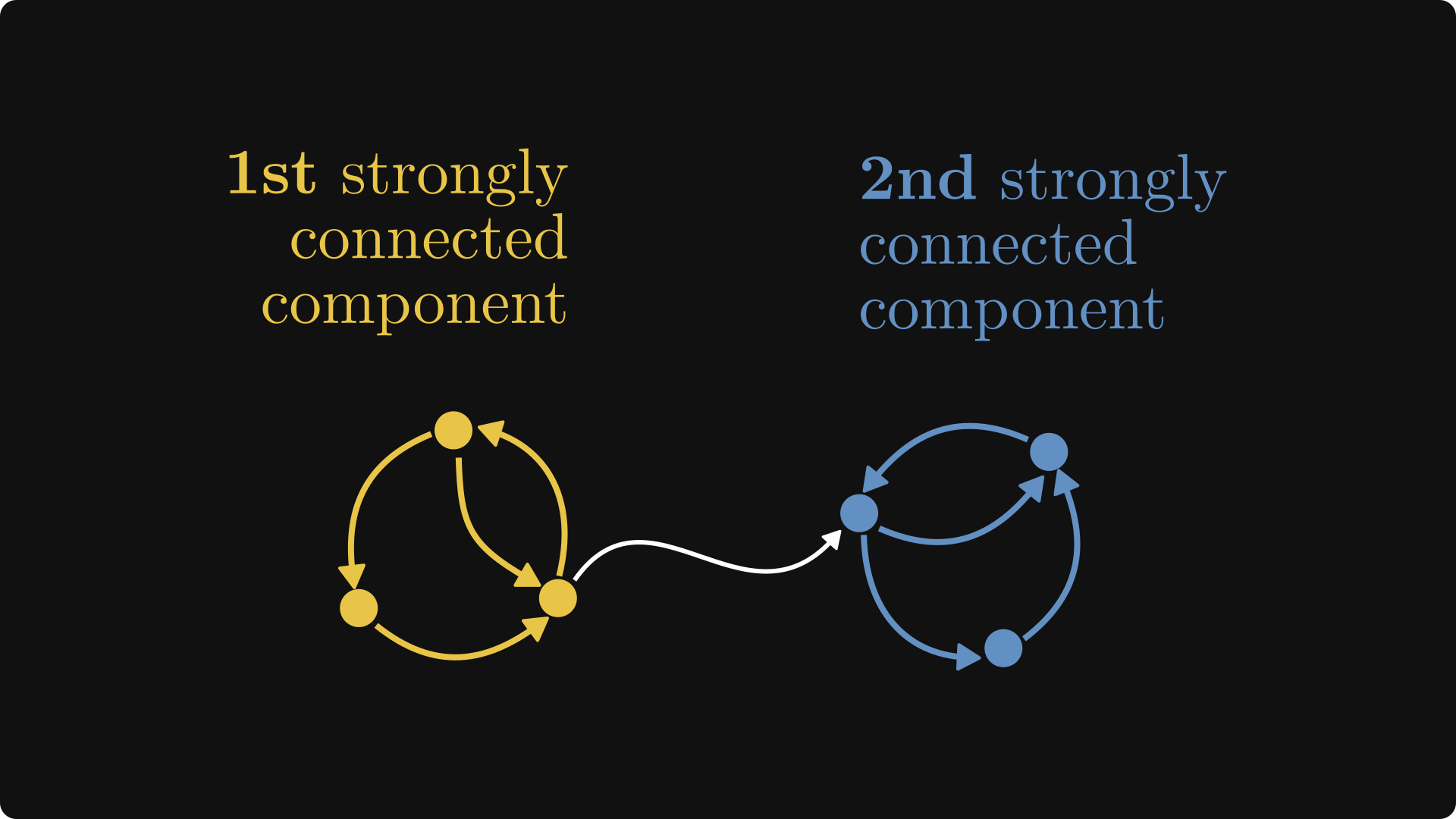
Even though not all directed graphs are strongly connected, we can partition the nodes into strongly connected components.
Let's label the nodes of this graph and construct the corresponding matrix!
(For simplicity, assume that all edges have unit weight.) Do you notice a pattern?
The corresponding matrix of our graph can be reduced to a simpler form!
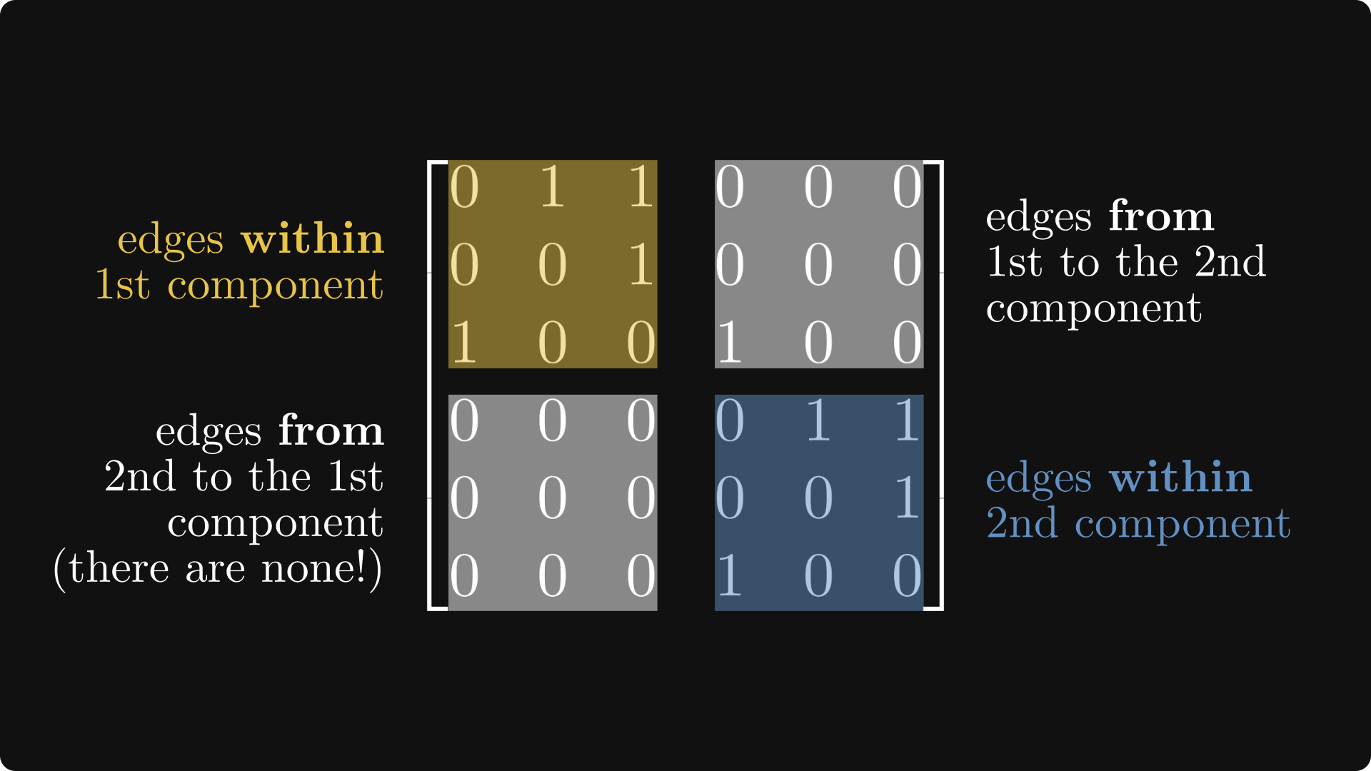
Its diagonal comprises blocks whose graphs are strongly connected. (That is, the blocks are irreducible.) Furthermore, the block below the diagonal is zero.
Is this true for all nonnegative matrices?
You bet. Enter the Frobenius normal form.
The Frobenius normal form
In general, this block-matrix structure that we have just seen is called the Frobenius normal form.
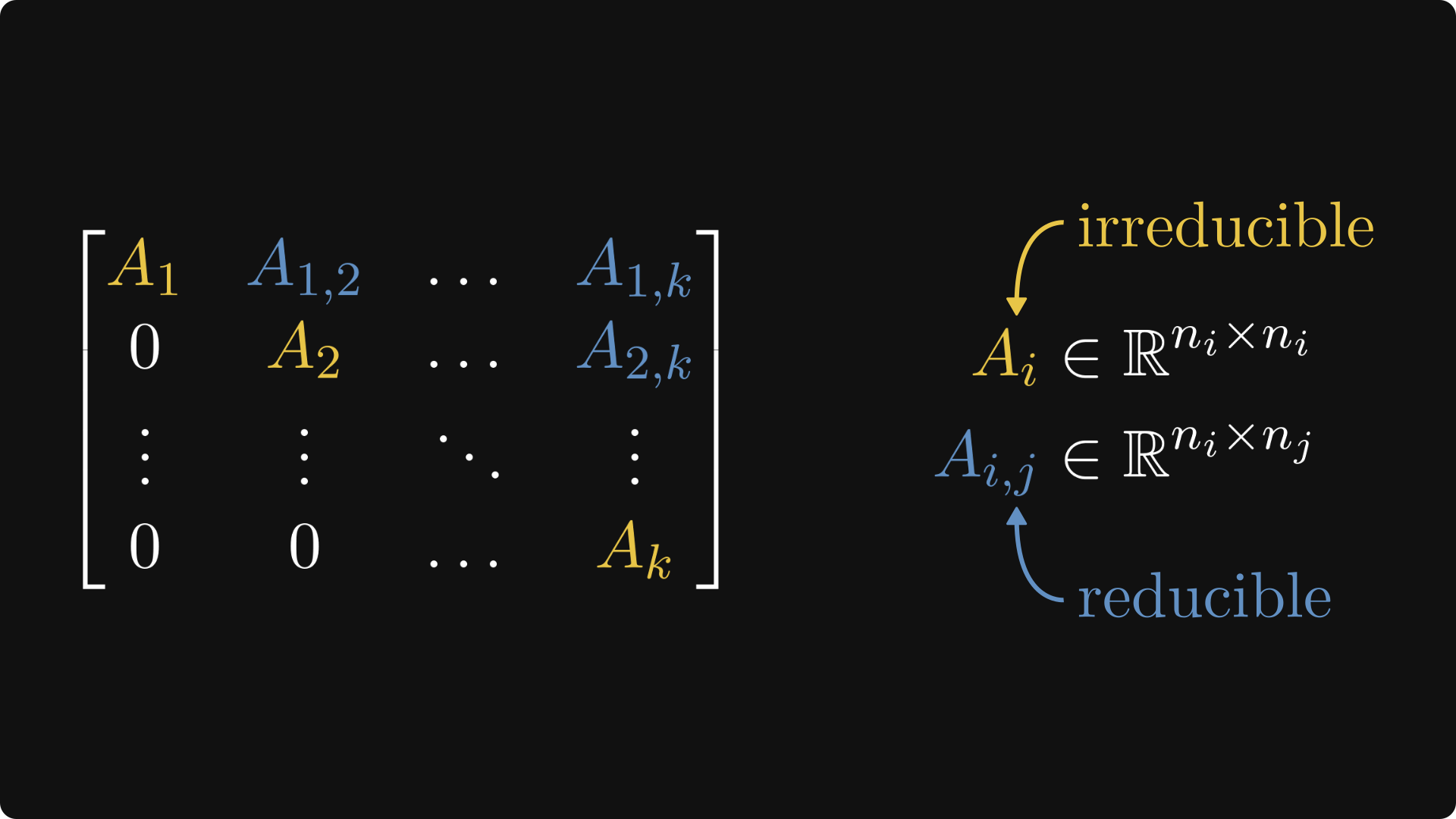
If you have a sharp eye with a hint of OCD, you probably noticed that I switched up the colors a bit. From now on, irreducible blocks (a.k.a. matrices that correspond to strongly connected graphs) will be colored maize, while reducible ones will be light blue.
Let's reverse the question: can we transform an arbitrary nonnegative matrix into the Frobenius normal form?
Yes, and with the help of directed graphs, this is much easier to show than purely using algebra.
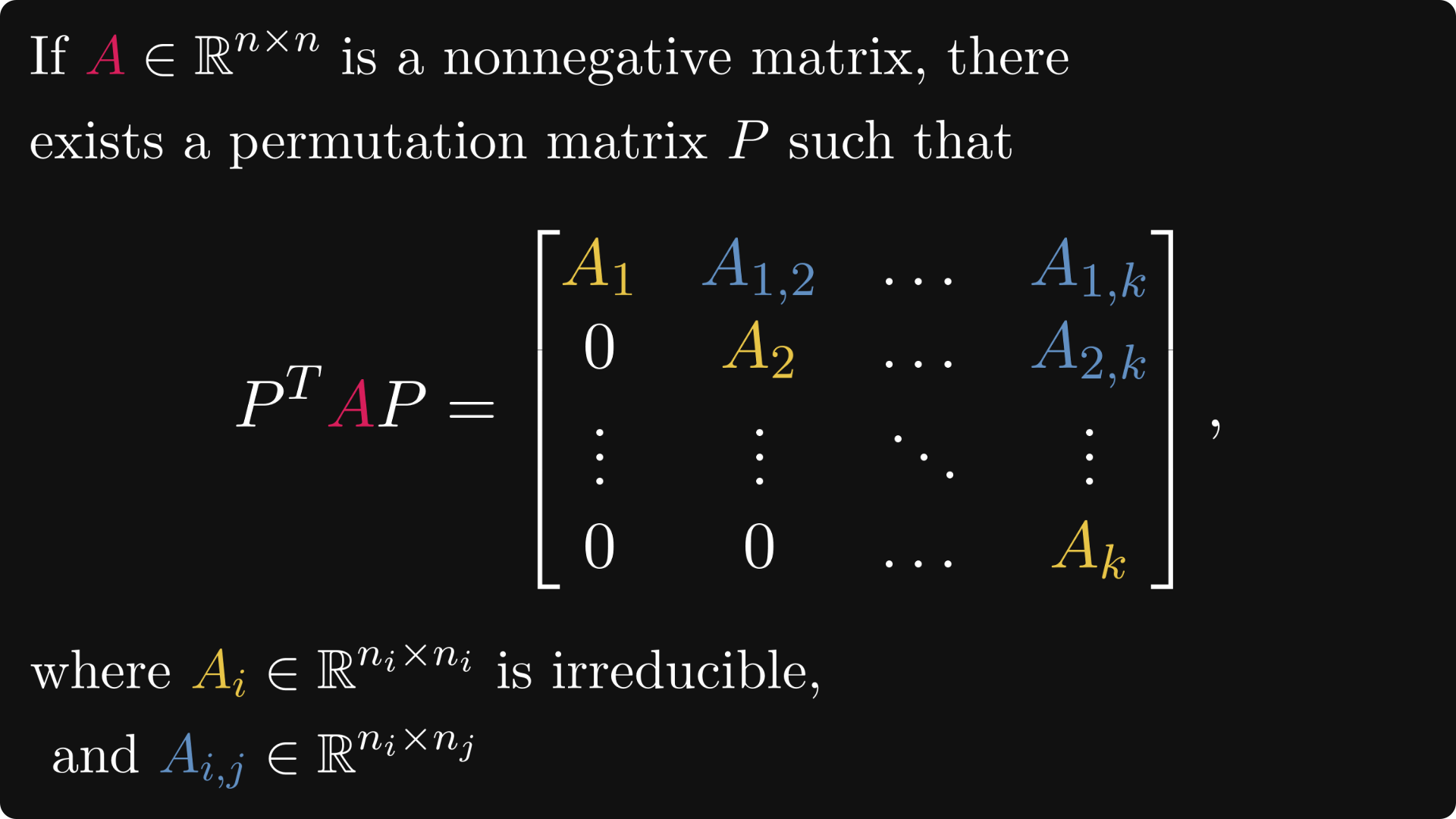
Here is the famous theorem in full form.
But what are permutation matrices?
Permutation matrices
Let’s look at a special case: what happens if we multiply a 2 x 2 matrix with
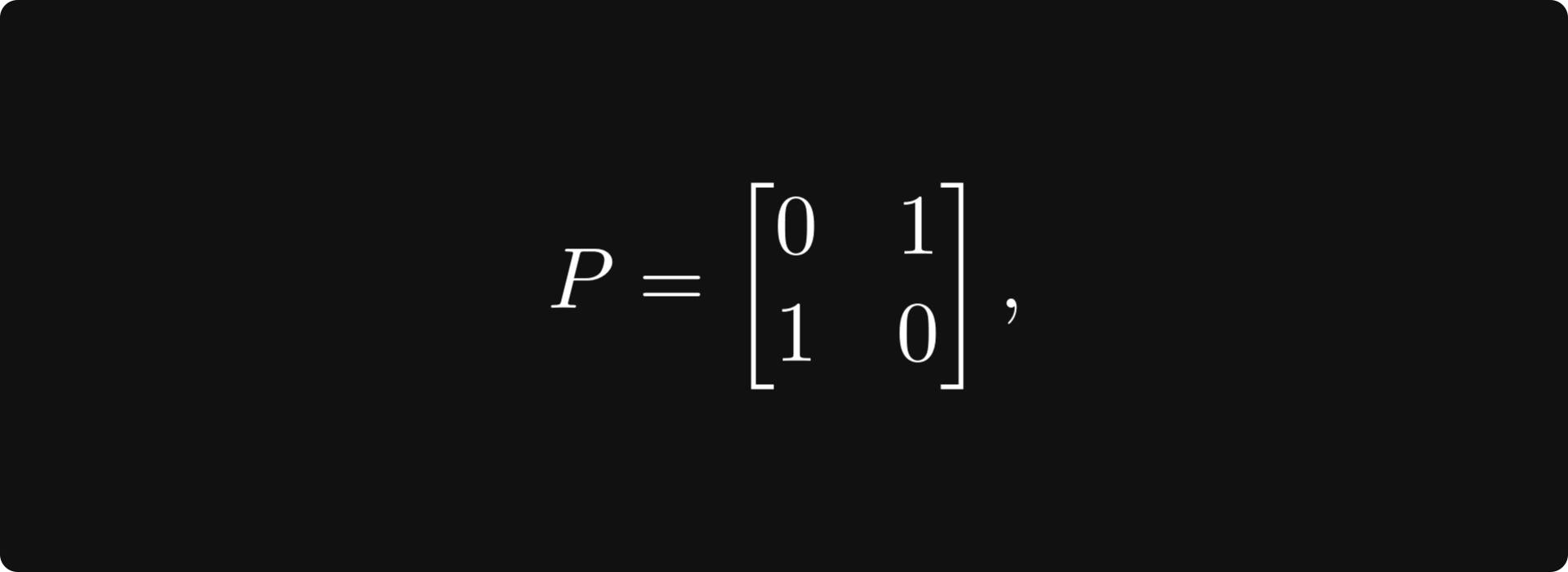
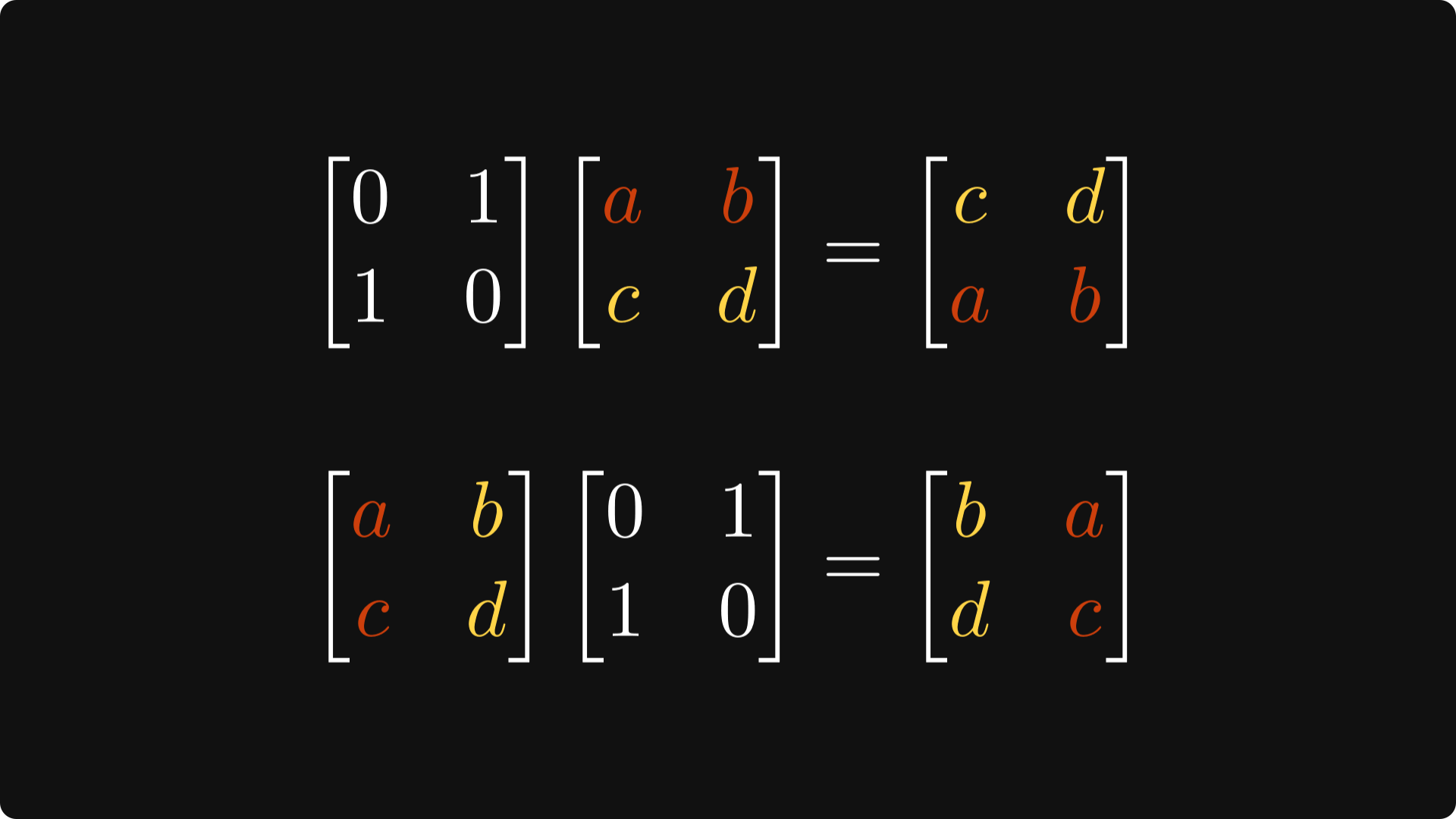
a simple zero-one matrix? With a quick calculation, you can verify that
it switches the rows when multiplied from the left,
and it switches the columns when multiplied from the right.
Just like this:
Multiplying with P from both left and right compounds the effects: it switches rows and columns.
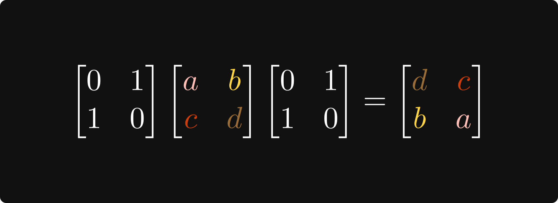
(By the way, this is a similarity transformation, as our special zero-one matrix is its own inverse. This is not an accident; more about it later.)
Why are we looking at this? Because behind the scenes, this transformation doesn’t change the underlying graph structure, just relabels its nodes!
You can easily verify this by hand, but I visualized it for you below.

A similar phenomenon is true in the general n x n case. Here, we define the so-called transposition matrices by switching the i-th and j-th rows of the identity matrix:
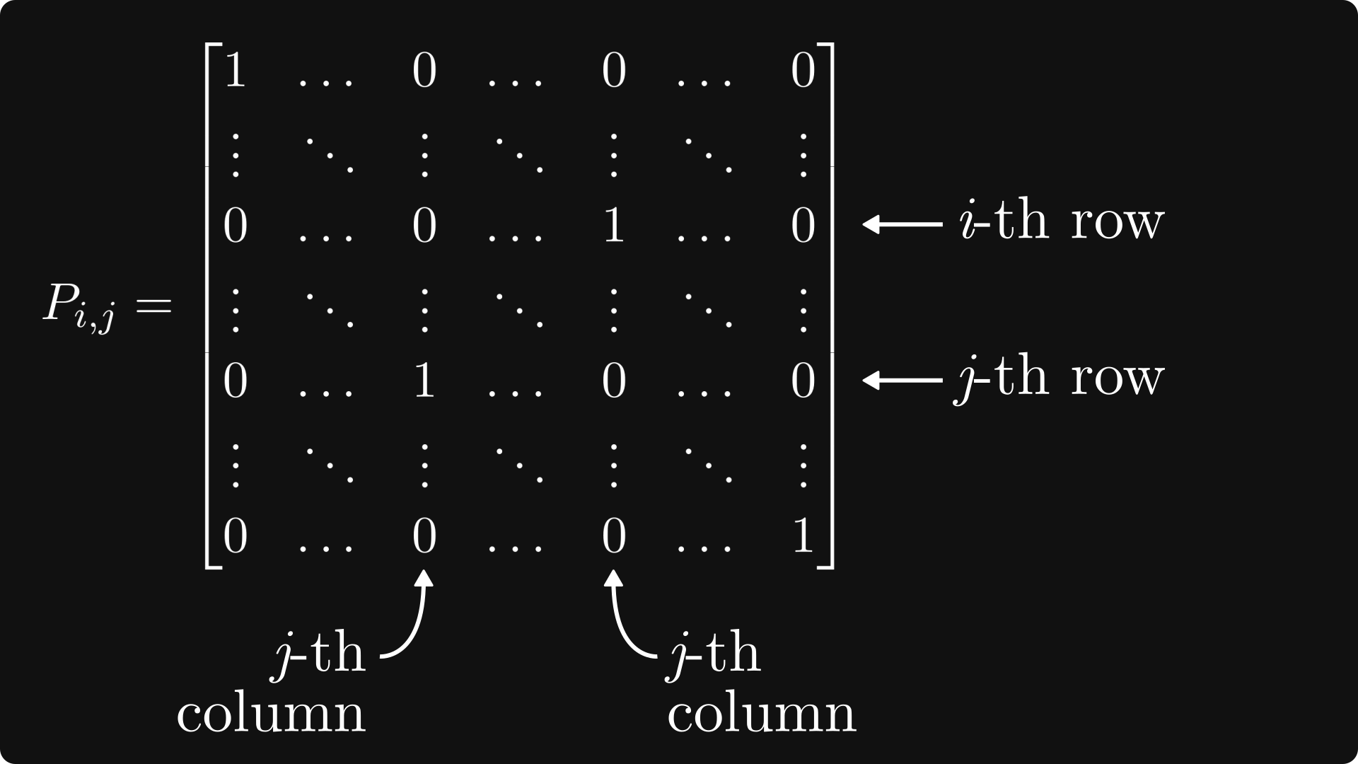
Multiplication with a transposition matrix has the same effect: switches rows from the left, and switches columns from the right.
We are not going to spell it out in detail (as the overcomplicated notation makes it especially painful), but you can verify by hand that this is indeed what’s going on.
Here is a brief summary. Take note of these, as they’ll be essential in a bit.

The most important property for us: similarity transformations with transposition matrices just relabel two nodes, but otherwise leave the graph structure invariant.
Now, about the aforementioned permutation matrices. A permutation matrix is simply a product of transposition matrices.

Permutation matrices inherit some properties from their building blocks. Most importantly,
their inverse is their transpose,
and a similarity transformation with them is just a relabeling of nodes that leave the graph structure invariant.
To see this latter one, consider the following argument below.
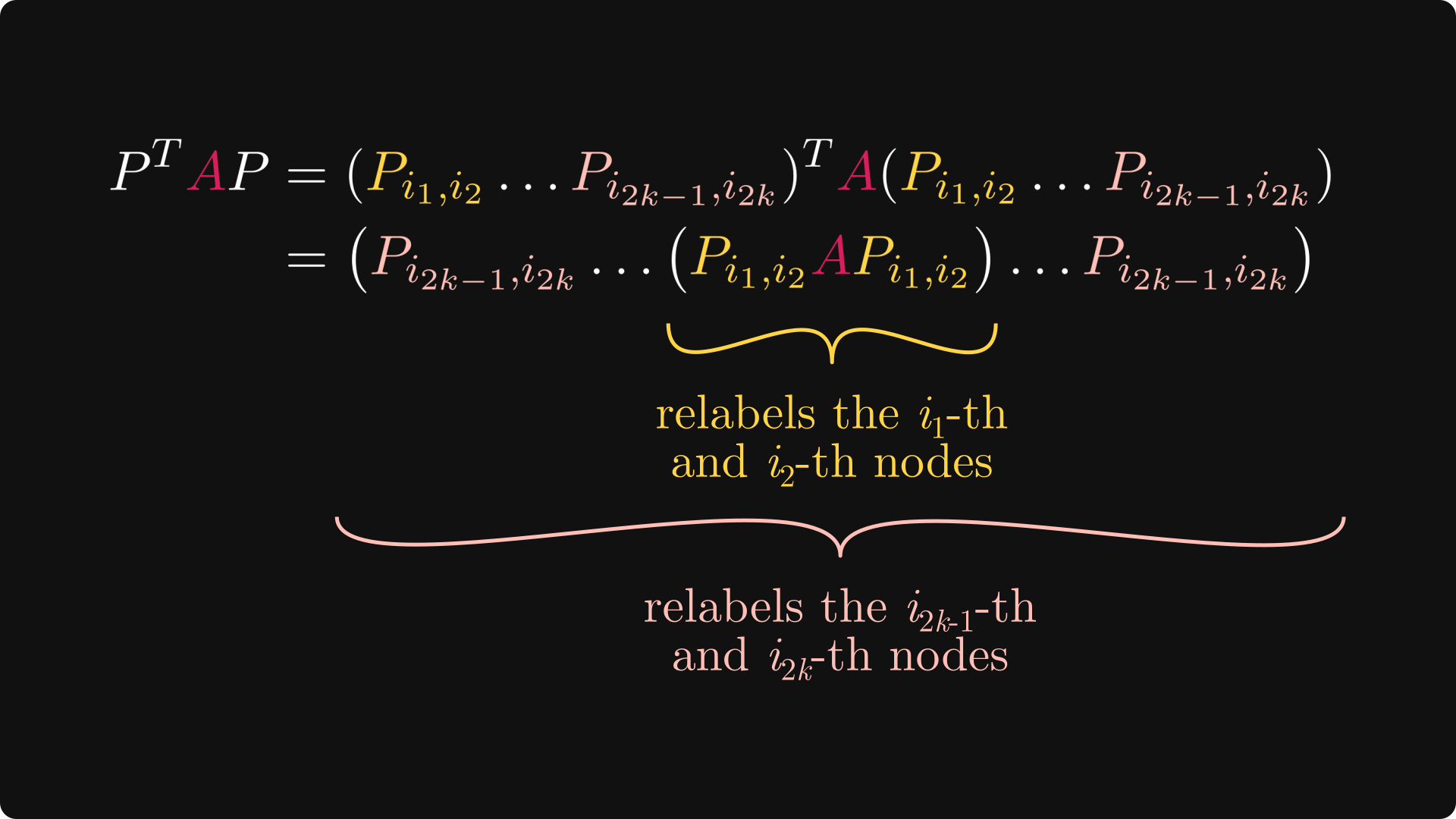
(Recall that transposing a matrix product switches up the order, and transposition matrices are their own transposes.)
Conversely, every node relabeling is equivalent to a similarity transformation with a well-constructed permutation matrix.
Why are we talking about this? Because the proper labeling of nodes is key to the Frobenius normal form.
Directed graphs and their strongly connected components
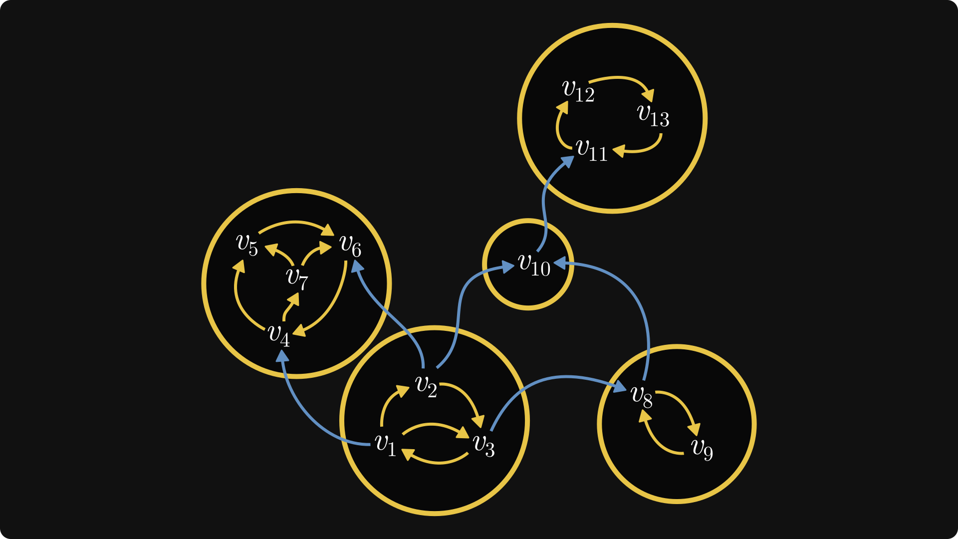
Now, let’s talk about graphs. We’ll see how every digraph decomposes into strongly connected components. For that, let’s see a concrete one.
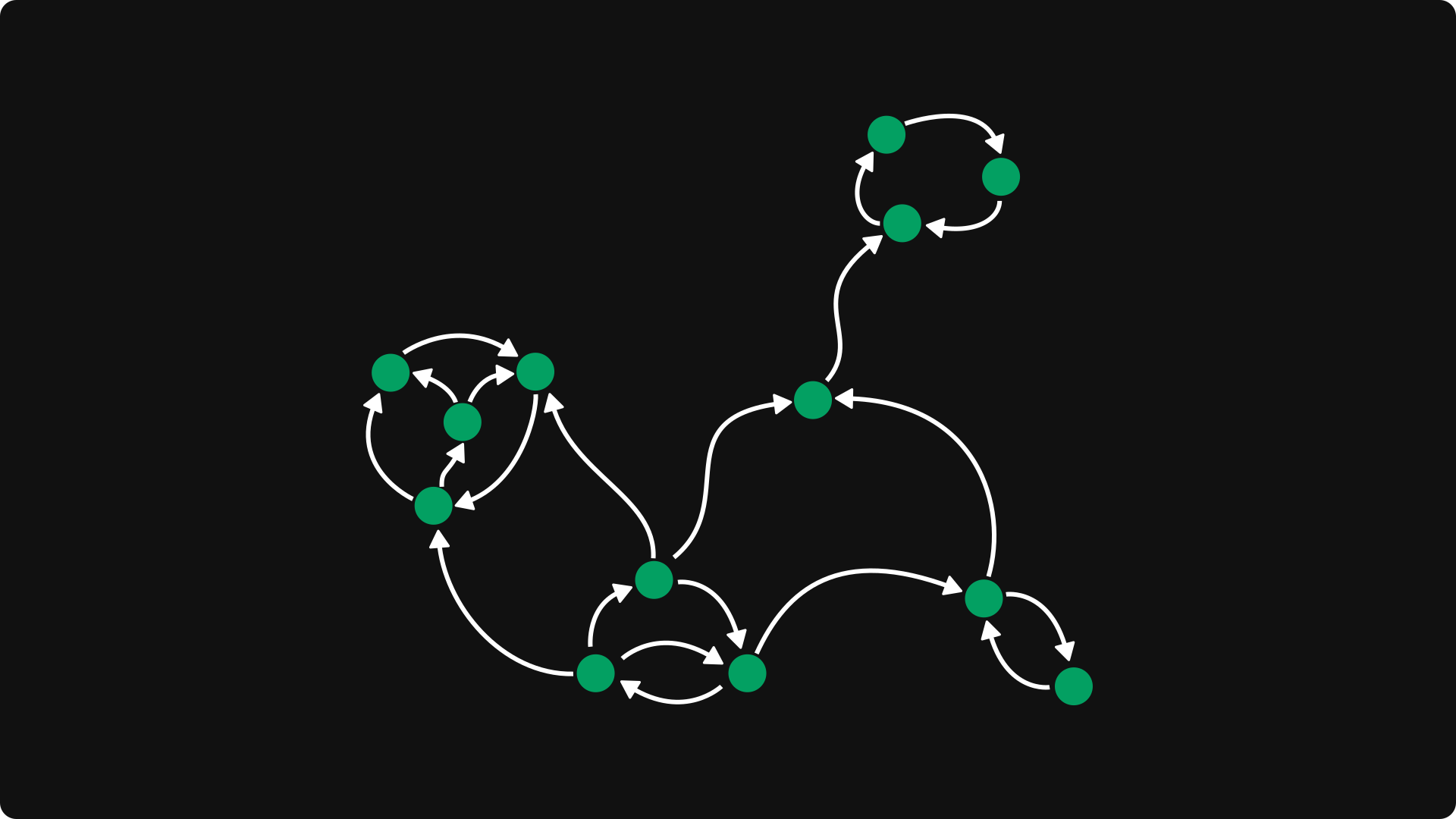
This’ll be our textbook example.
How many nodes can be reached from a given node? Not necessarily all. Say, for the one at the bottom right, only a portion of the graph is accessible.

However, the set of mutually reachable nodes is much smaller.
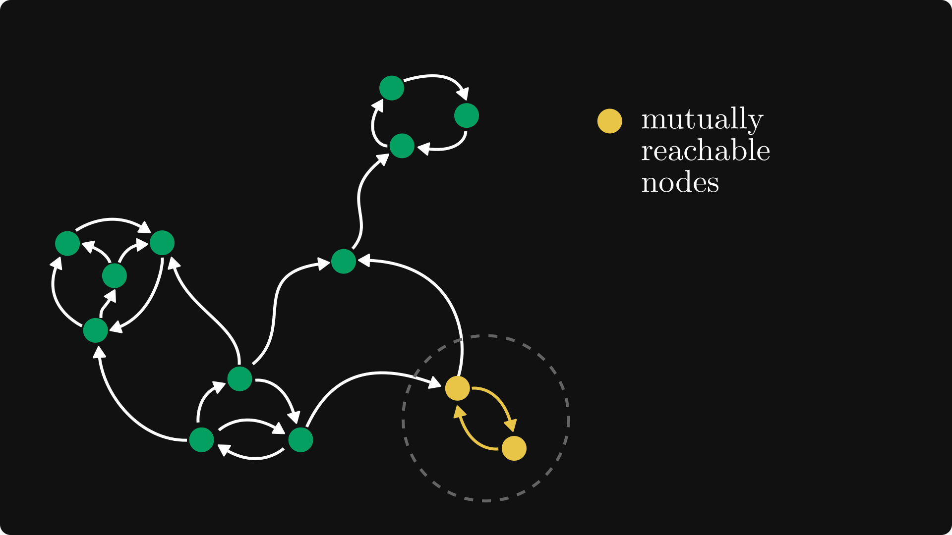
Algebraically speaking, the relation “a and b are mutually reachable from each other“ is an equivalence relation. In other words, it partitions the set of nodes into disjoint subsets such that
two nodes from the same subset are mutually reachable from each other,
and two nodes from different subsets are not mutually reachable.
(Equivalence relations are the workhorses of mathematics. If you are not familiar with them, check out this Wikipedia article about partitions to see how they relate.)
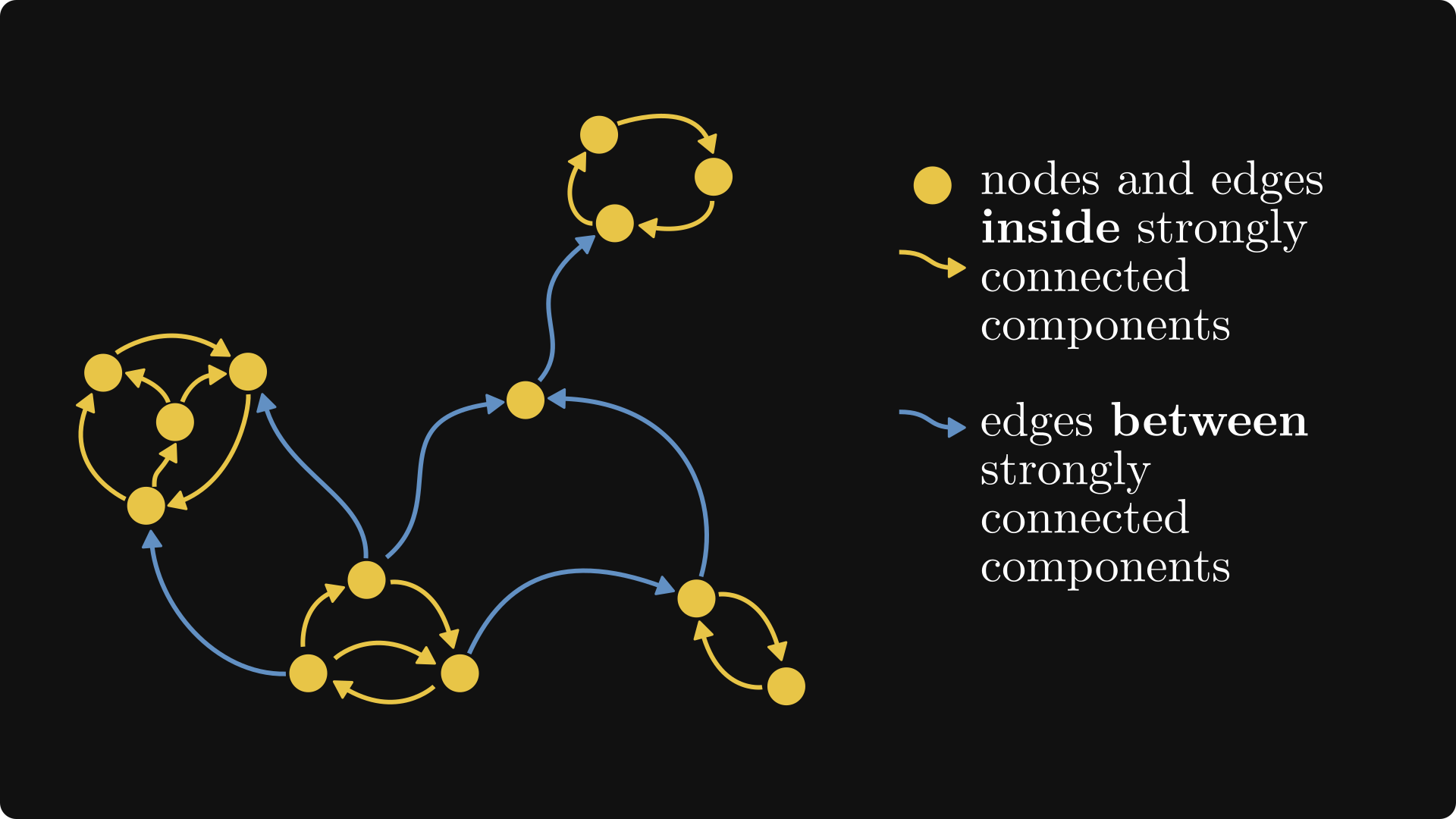
The subsets of this partition are called the strongly connected components, and we can always decompose a directed graph in this way.
Now, let’s connect everything together! (Not in a graph way, but you know, in a wholesome mathematical way.)
Putting graphs and permutation matrices together
We are two steps away from proving that every nonnegative square matrix can be transformed into Frobenius normal form with a permutation matrix.
Here is the plan.
Construct the graph for our nonnegative matrix.
Find the strongly connected components.
Relabel the nodes in a clever way.
And that’s it! Why? Because, as we have seen, relabeling is the same as a similarity transform with a permutation matrix.
There’s just one tiny snag: what is the clever way? I’ll show you.
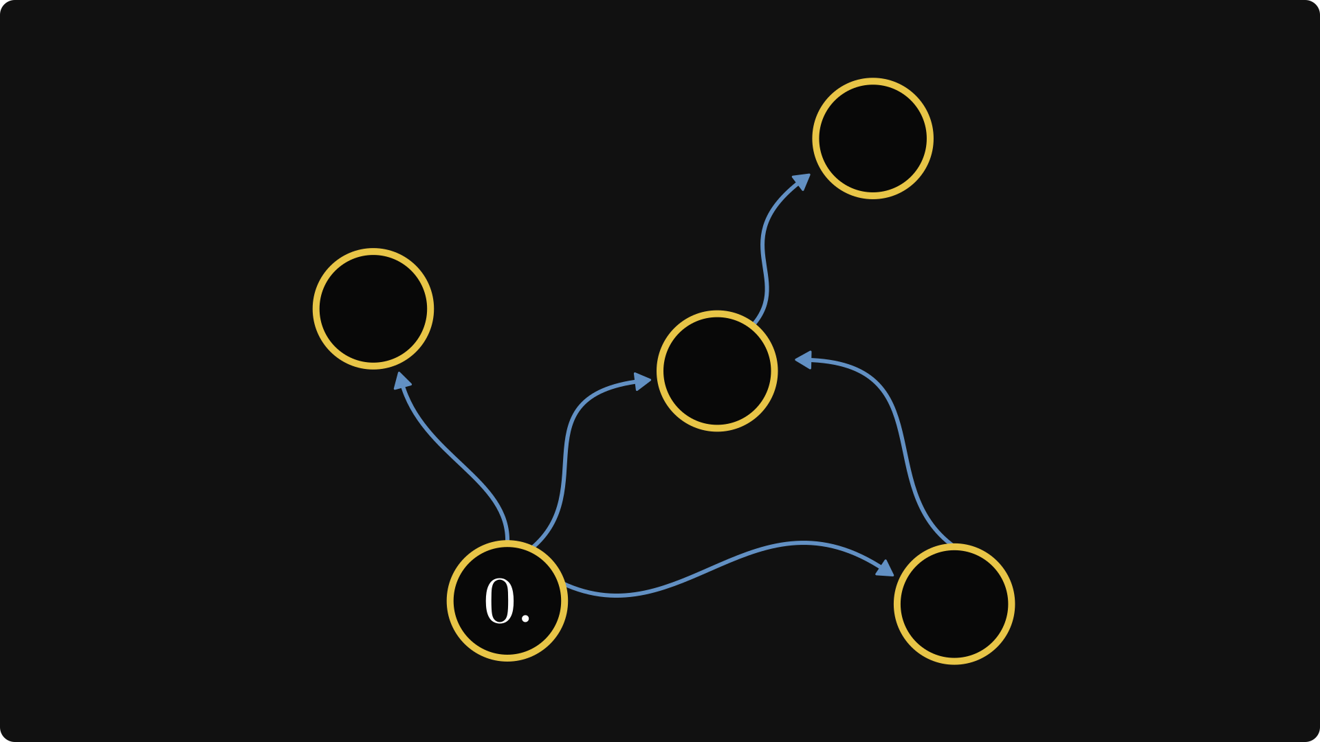
First, we “skeletonize” the graph: merge the components together, as well as any edges between them. Consider each component as a black box: we don’t care what’s inside, only about their external connections.
In this skeleton, we can find that components that cannot be entered from another components. These will be our starting points, the zeroth-class components. In our example, we only have one.
Now, things get a bit tricky. We number each component by the longest path from the farthest zero-class component from which it can be reached.
This is hard to even read, let alone to understand. So, here is what’s happening.

The gist is that if you can reach an m-th-class from an n-th-class, then n < m.
In the end, we have the following.
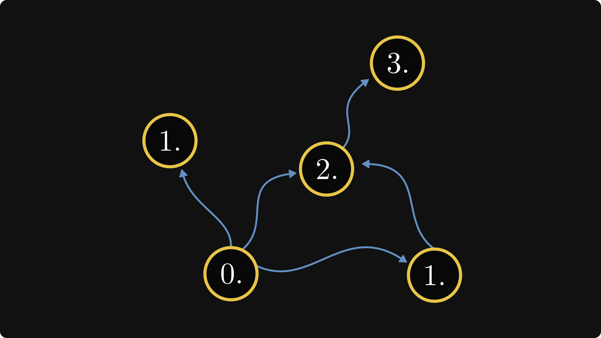
This defines an ordering on the components. (A partial ordering, if you would like to be precise.)
Now, we label the nodes inside such that
higher-order classes come first,
and consecutive indices are labeling nodes from the same component if possible.
This is how it goes.
If the graph itself is coming from an actual matrix, such a relabeling yields the Frobenius normal form!
Here is the matrix in this particular example, with zeros and ones for simplicity:

Now we have everything, and the “proof” behind the transformation to Frobenius normal form is complete!
To remind you, this is the theorem in its full form:

Conclusion
What we have seen is just the tip of the iceberg. For example, with the help of matrices, we can define the eigenvalues of graphs! This idea gave birth to the fascinating topic of spectral graph theory, a beautiful field of mathematics.
Utilizing the relation between matrices and graphs has been extremely profitable for both graph theory and linear algebra.
If you are interested in the details, I have two books to recommend to you. One is the fantastic A Combinatorial Approach to Matrix Theory and Its Applications by Richard A. Brualdi and Dragos Cvetkovic, my favorite learning resource on the topic.
Second, I recently finished writing my Linear Algebra for Machine Learning book. Although the contents of this post are not yet a part of this, the good thing about the ebook format is that I can always go back and add a new chapter here and there.
So, I am planning to expand this post into a textbook-like chapter, possibly with interactive code examples along the way. If you are interested, check out the first two chapters of my book!
I was thinking of this passage: "we define the so-called transposition matrices by switching the i-th and j-th rows of the identity matrix". If it's the identity matrix, then it has 1s on the diagonal everywhere but on lines i and j I suppose. It caught my eye because otherwise I don't see how P^2 = I could work out.
Fascinating post, many thanks!
If I understood correctly, it doesn't matter whether the nonnegative matrix A is irreducible or not, it always has a Frobenius normal form. However, is irreducibility (or reducibility) of A somehow reflected in the normal form?